In-Depth Explanation of the Hjulström Diagram

Introduction and Background

The Hjulström Diagram is a graphical representation that illustrates how different sizes of sediment grains interact with a moving fluid – typically water. Formulated by Filip Hjulström in 1935, this diagram establishes the critical threshold velocities needed for sediment particles to be eroded from the bed, transported along as bedload or suspended load, and finally deposited when the flow energy drops. In sedimentary processes, understanding these thresholds is vital as it determines the sorting, deposition, and overall stratigraphic characteristics of sedimentary rocks, which in turn influence subsurface reservoir quality.

While the diagram itself is a simplified representation, it encapsulates many fundamental aspects of sediment transport. In particular, the diagram shows three main processes: erosion, transport, and deposition – each governed by the combined effect of water velocity and sediment size.

The Diagram Layout and Axes

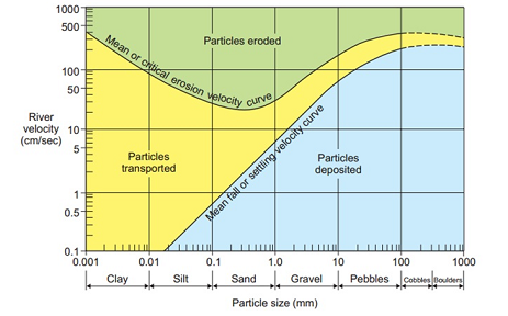
The diagram typically consists of two axes:

Horizontal Axis (X-axis): Represents the size of sediment particles. This axis is usually logarithmic to capture a wide range of grain sizes, from fine clays (micrometers) to coarse gravels (millimeters to centimeters).
Vertical Axis (Y-axis): Represents the flow velocity (often in centimeters per second), which is the speed of the water moving over the sediment surface.

These axes help define critical thresholds where the moving water can:

Erode sediment from the bed.
Transport sediment particles by either rolling them along the bed (bedload) or keeping them in suspension (suspended load).
Deposit sediment when the water’s velocity falls below a certain threshold.

        Note: In the diagram, for a given sediment grain size, a higher water velocity is required to erode the grain compared to the velocity required to simply maintain it in suspension.
      

Concepts and Processes Illustrated by the Diagram

Erosion: This is the process by which sediment is lifted off the bed of a river or stream. In the Hjulström Diagram, the erosion curve is plotted, indicating that only when the flow velocity exceeds a critical value can it overcome the forces binding the sediment to the bed. For example, cohesive sediments like clay require much higher velocities for erosion even though, once in suspension, they can remain aloft at very low velocities.

Transport: Once sediment is loosened, it can be transported in the flow in two main ways:

As bedload: Larger particles (e.g., sand or gravel) roll, slide, or bounce along the bottom.
As suspended load: Finer particles (e.g., silt and clay) are kept in suspension by the turbulent energy of flowing water.

The diagram shows the velocities that enable particles of different sizes to remain in suspension. Note that even though fine particles are easier to lift, they also tend to settle quickly if the velocity decreases beneath a certain threshold.

Deposition: When the flow velocity falls below what is required to support the sediment in suspension, particles begin to settle and accumulate. The deposition curve in the diagram marks this threshold, signifying the point where sediment deposition occurs. Deposition is a key process in forming sedimentary layers, which later become sedimentary rocks.

Important Assumption: The diagram assumes a uniform flow condition and does not fully account for complex variables such as sediment shape, water temperature, and chemical composition. However, it remains an effective visual abstraction of sediment transport dynamics.

Mathematical Insight and Threshold Concepts

While the Hjulström Diagram is primarily a conceptual tool, it often implies underlying mathematical relationships between the shear stress, sediment particle weight, and fluid dynamics. The key mathematical idea involves comparing the drag force from the moving water against the gravitational force holding the particle at rest. In simple terms:

Drag force ∝ V² × Area

and the gravitational force can be approximated by:

Gravitational force ∝ (ρ_particle - ρ_fluid) × D³

Here:

V is the velocity of the fluid,
ρ_particle and ρ_fluid are the densities of the sediment particle and fluid respectively,
D represents the diameter (or characteristic size) of the particle.

By equating the drag force and gravitational force, one obtains an expression for the critical velocity (V_crit) required for erosion:

$V_{crit} ∝ ( (ρ_{particle} - ρ_{fluid}) × D )^{1/2}$

This simplification shows that critical velocity increases with particle size and the density contrast between the particle and the fluid. Fine particles, especially clays with high cohesiveness, require a significantly high velocity to be mobilized, even though they are very small in size. Conversely, once these particles are picked up, they remain suspended at much lower velocities.

        Side Note: The above relation is a simplification and in detailed sediment transport models, additional friction coefficients and fluid dynamic adjustments are introduced.
      

Application and Relevance in Sedimentary Processes

The Hjulström Diagram elegantly encapsulates the dynamic equilibrium between erosional and depositional forces. Its applications in sedimentology include:

Predicting Sediment Sorting: The diagram explains why high-energy environments (e.g., swiftly flowing rivers) often transport coarser material while low-energy environments (e.g., backwater zones) accumulate finer sediments.
Understanding Depositional Environments: By interpreting the flow velocities and sediment types present, geologists can reconstruct the environmental history of an area. For instance, the transition from high velocities (indicative of erosion) to low velocities (leading to deposition) suggests a change in the depositional setting, such as a river entering a delta.
Reservoir Quality Prediction: In petroleum geology, the distribution and sorting of grains influence the porosity and permeability of reservoir rocks. By utilizing insights from the Hjulström Diagram, geologists can predict where high-quality reservoirs are likely to form.

For example, a sand deposit that forms in an area characterized by just enough velocity to maintain transport but eventually falls below the deposition threshold will result in well-sorted, well-cemented sandstone. This makes it a prime candidate as a reservoir, as good sorting typically results in high porosity.

Assumption Reminder: The diagram is based on idealized conditions. Actual sedimentary environments can be influenced by tides, waves, and variable sediment supply which may alter the thresholds.

Detailed Process Walkthrough

Let us take a detailed walk-through of the sediment transport process using the Hjulström Diagram:

Step 1: Initial Erosion
Imagine a river with a high flow velocity. For a given large grain size, the flow must exceed the critical threshold (as indicated by the diagram) to dislodge the sediment from the river bed. Here, the water’s kinetic energy overcomes the gravitational and cohesive forces binding the sediment. This condition is plotted above the erosion curve.
Step 2: Transition to Transport
Once eroded, the sediment is entrained in the flow. Depending on its size, it might immediately join the bedload (rolling along the bottom) or get lifted into the water column as suspended load. The diagram reflects that for smaller particles, even moderate velocities can maintain suspension.
Step 3: Deposition
As the river encounters a zone of lower energy—perhaps because of a reduction in slope or the entry into a wider channel—the flow velocity decreases. When this velocity falls below the deposition threshold outlined by the diagram, the sediment particles begin to settle out. In a natural setting, this may lead to the formation of distinct stratified layers or graded bedding observed in sedimentary rocks.

Each of these steps is essential to forming the stratigraphic record that geologists study. The Hjulström Diagram helps predict where the boundaries between these layers may occur based on changes in flow velocity and sediment size.

Key Takeaways and Summary

To encapsulate, the Hjulström Diagram provides an intuitive framework for understanding sediment transport dynamics. The major points include:

There is a critical flow velocity required to initiate erosion, which increases with grain size and depends on factors like cohesion and density differences.
Once sediment is in motion, finer particles can be maintained in suspension at low velocities while coarser sediments require higher velocities as bedload.
Deposition occurs when the flow energy decreases below the threshold necessary to keep particles in suspension, leading to the formation of sediment layers.
This balance between erosion, transport, and deposition governs the architecture of sedimentary deposits, influencing sedimentary facies and reservoir quality.

Thus, by analyzing the interplay of these factors as depicted in the Hjulström Diagram, sedimentologists and petroleum geologists are better equipped to interpret past depositional environments and predict rock properties that control fluid flow in reservoirs.

        Remember: The diagram is a simplification. While it provides a strong conceptual framework, detailed field measurements and additional modeling are necessary for precise predictions.
      

Concluding Remarks

The Hjulström Diagram continues to be a cornerstone in sedimentary geology. Its strength lies in its ability to visually correlate sediment size with flow velocity, thereby offering insights into both the natural processes that form sedimentary rocks and the factors that define reservoir quality. Understanding and applying this diagram allow geoscientists to bridge the gap between observable sedimentary structures and the dynamic processes in modern fluvial, deltaic, and marine environments.

In summary, the diagram not only serves as a teaching tool but also as a practical model that informs decisions in exploration and production of subsurface resources. It emphasizes the necessity of considering both physical forces and sediment characteristics when evaluating sediment transport and deposition.